Common methods
This section describes the ML and DL architectures employed for HAR classification and the statistical tools used to determine the significance of the presented results that will be used in the following sections.
ML and DL
In the context of HAR and thoroughout this thesis, labelled data is employed to train ML or DL models and to determine –classify– the activity a user is performing given some input data. Therefore, this dissertation faces a supervised learning classification problem.
Next, the models employed, the evaluation metrics used to evaluate them and the tools used to develop them are described.
Models employed
Multilayer Perceptron (MLP)
The Perceptron was invented by McCulloch and Pitts (1943), inspired by the neurons present in the brain, which receive, process and transmit information. Rosenblatt (1958) implemented the first Perceptron with learning capabilities, where a neuron would receive a series of inputs in the input layer. These inputs would be combined through a weighted sum and passed through an activation function, generating an output in the output layer. However, the Perceptron presented an issue: it could only solve problems with linear solutions.
A solution for this problem was proposed with the MLP, which consisted of stacking several perceptions. However, the learning ability in these MLP was not possible until the development of the Backpropagation algorithm. The MLP is usually fed with features extracted from raw data after a feature engineering process into an input layer, multiple hidden layers and an output layer. Since feature engineering is required, MLP are considered ML techniques.
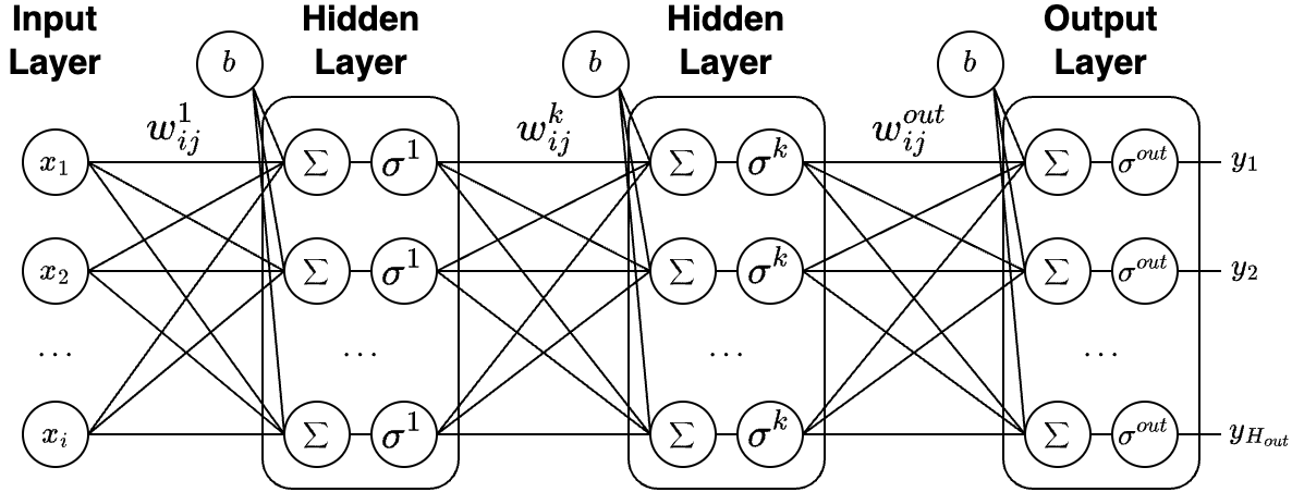
Figure 5.1 shows the architecture of an MLP. Each layer contains a set of neurons, and each neuron is connected to the neurons in the next layer with a weight (parameters of the network). The outputs of the first hidden layer can be formulated as: \[\begin{equation} h_i^1 = \sigma^1(b+\sum^{H_1}_{j=1}w_{ij}^1x_i)\,, \end{equation}\] where \(x_i\) is the \(i^{th}\) input, \(w_{ij}^1\) is the weight of the connection between \(x_i\) and the \(j^{th}\) neuron in the layer, \(b\) is a constant bias not affected by the previous layer, \(H_1\) is the amount of neurons in the layer and \(\sigma^1\) is the activation function. Given \(k\) layers, the equation can be generalized as follows: \[\begin{equation} h_i^k = \sigma^k(b+\sum^{H_k}_{j=1}w_{ij}^kh_i^{k-1})\,. \end{equation}\]
The results of the output layer can also be expressed as follows: \[\begin{equation} y_i = \sigma^{out}(b+\sum^{H_{out}}_{j=1}w_{ij}^{out}h_i^{k})\,. \end{equation}\]
Convolutional Neural Network (CNN)
Fukushima (1980) invented the Neocognitron for vision-based pattern recognition, inspired by the work of (Hubel and Wiesel 1959), who showed that individual cells on the visual cortex respond to small regions of the visual field and that neighbouring cells have similar and overlapping receptive fields. Then, Atlas, Homma, and Marks (1987) proposed replacing the multiplications inside a neuron with a convolution, a computation between a small area (receptive field) and a filter containing the trainable weights of the network.
These networks are the CNN and contain convolution layers, which are useful for feature recognition in data with spatial and temporal domains. These networks have diverse applications, such as vision applications or time series prediction. They can be directly fed with raw data (i.e., no need for feature extraction), and therefore, are considered as DL techniques.
The convolutional layers apply a set of convolutional kernels (learnt during training) to an input to obtain an output. These kernels \(K\in R^{i\times j}\) are applied to an input matrix \(A\in R^{x\times y}\) sliding them over its width and height computing the convolution operation over each data point, obtaining as a result a new matrix \(B\in R^{m\times n \times d}\), where \(m=x-i+1\), \(n=y-j+1\) and \(d\) is the number convolutional kernels applied. For 1 and 2-dimensional convolutions, the result for \(B_{(m,n)}\) is defined as an element-wise multiplication, or: \[\begin{equation} B_{(m,n)} = \sum_i\sum_j A_{(m+i,n+j)}K_{(i,j)}\,. \end{equation}\]
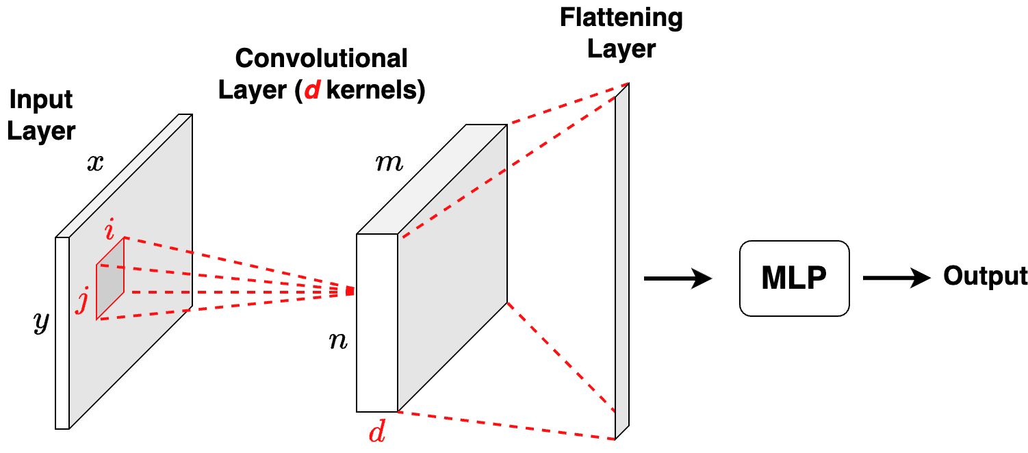
Figure 5.2 shows the architecture of a CNN network. Since the convolutional layers act as feature extractors, these networks add after the convolutional layers and a flattening layer to reduce the convolved output to one dimension, a classifier or a regressor (e.g., MLP).
Long-Short Term Memory (LSTM)
When the data has a sequential nature (e.g., time-series), RNN can be useful since they can remember information from the previous status and use it for the current status. This is possible because the output of specific neurons can be employed as subsequent input of the same neurons. However, the learning, driven by the backpropagation algorithm, suffers from several issues such as the vanishing and exploding gradient.
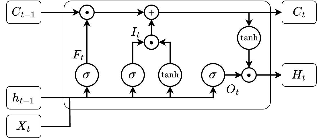
To solve these issues, Hochreiter and Schmidhuber (1997) invented the LSTM architecture, consisting of LSTM cells. An LSTM cell receives as input the state (\(C_{t-1}\), or long-term memory) and hidden state (\(H_{t-1}\), or short-term memory) of the previous cell at instant \(t-1\), and an input vector (\(X_{t}\)) at the current instant (\(t\)). Its outputs are the state (\(C_t\)) and the hidden state (\(H_t\)). Since the input vectors are raw sequences, they are considered DL techniques. While LSTM networks are usually used for forecasting, they can also be combined with classifiers (i.e., MLP) to solve such tasks.
The architecture of the LSTM cell is depicted in Figure 5.3. Internally, the cell is composed of three gates (i.e., neural networks):
- Forget gate (\(F_t\), Equation 5.1): determines based on \(X_t\) and \(H_{t-1}\) (short-term memory) what information must be removed (i.e., forgotten) from the state at the previous instant (\(C_{t-1}\), long-term memory).
- Input gate (\(I_t\), Equation 5.2): determines based on \(X_t\) and \(H_{t-1}\) what information must be included (i.e., remembered) in the cell state (\({C_t}\)). The updated \(C_{t}\) Equation 5.4 will be used for the cell at \(t+1\).
- Output gate (\(O_t\), Equation 5.3): determines based on \(H_{t-1}\) and \(C_{t}\) what information must be kept in \(H_{t}\) Equation 5.5 and used for the LSTM cell at \(t+1\).
\[ F_t=\sigma(W^X_FX_t + W^{h_{t-1}}_Fh_{t-1} + b_F)\,. \tag{5.1}\]
\[ I_t=\sigma(W^X_IX_t + W^{h_{t-1}}_Ih_{t-1} + b_I) \cdot \tanh(W^X_CX_t + W^{h_{t-1}}_Ch_{t-1} + b_C)\,. \tag{5.2}\]
\[ O_t=\sigma(W^X_OX_t + W^{h_{t-1}}_Oh_{t-1} + b_O)\,. \tag{5.3}\]
\[ C_t=C_{t-1} \cdot F_t + I_t\,. \tag{5.4}\]
\[ H_t=\tanh(C_t) \cdot O_t\,. \tag{5.5}\]
CNN Long-Short Term Memory (CNN-LSTM)
While the LSTM architectures are useful for modelling temporal dependencies, they do not leverage the spatial nature of the data. To address this issue several solutions were proposed, such as the ConvLSTM network which extends the LSTM by adding convolutional operations in the input and state-to-state transitions (Shi et al. 2015). Another approach was to join the CNN and the LSTM networks, in the so-called CNN-LSTM network to take advantage of the spatial and temporal modelling capabilities of both networks (Sainath et al. 2015). Like the CNN and LSTM, both networks are considered DL techniques.
In this dissertation, we employ the CNN-LSTM since it has shown similar and better results than the ConvLSTM in HAR and other fields while being less resource-consuming.
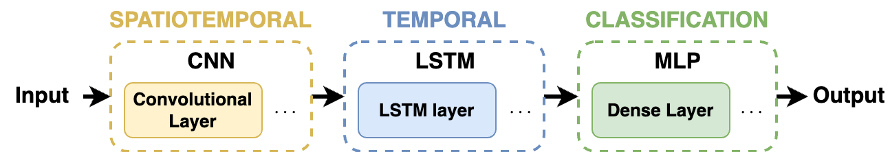
The architecture of the CNN-LSTM network is depicted in Figure 5.4. The input of the network consists of convolutional layers for spatiotemporal modelling. Then, the outputs of those convolutional layers go through several LSTM layers for modelling temporal dependencies. Finally, the outputs of the LSTM layers are fed into a MLP to perform classification.
Evaluation metrics
The performance of the ML and DL models can be measured in several ways. Along this thesis, we employ the accuracy, precision, recall and F1-score metrics
Accuracy
Measures the ratio between the correct and all the generated predictions. It allows to obtain an overall insight into the performance of the model.
\[ Accuracy=\frac{Correct~predictions}{All~predictions}\,. \]
Precision
The ratio between the correct predictions of a certain class \(A\) and all the generated predictions of class \(A\), whether they are correct or not. It answers the following question: how good is the model identifying samples of class \(A\)? Precision is defined by the following equation: \[ Precision_{A}=\frac{Correct~predictions~of~A}{All~predictions~of~A}=\frac{TP_{A}}{TP_{A} + FP_{A}}\,, \] where \(TP_{A}\) (true postives) is the number of correct preditions of class \(A\) and \(FP_{A}\) (false positives) is the number of samples wrongly predicted as class \(A\).
Recall
Measures the ratio between the correct predictions of class \(A\) and all samples that should be predicted as \(A\). It answers the following question: how good is the model to identify samples of class \(A\)? Recall is defined as: \[ Recall_{A}=\frac{Correct~predictions~of~A}{All~real~instances~of~A}=\frac{TP_{A}}{TP_{A} + FN_{A}}\,, \] where \(FN_{A}\) (false negatives) is the number of samples of class \(A\) classified to other classes.
F1-score
Measures the predictive performance of a model on specific classes taking into account the precision and the recall. It is defined as: \[ F1-score_{A}=2\frac{Precision_{A}*Recall_{A}}{Precision_{A}+Recall_{A}}\,. \]
Tools
The ML and DL models employed in the following chapters have been built in Python 3.9 using the Keras library under the TensorFlow v2.10.0 backend.
In addition, this thesis contributes to the AwarNS Framework by developing a package to run ML and DL models in a smartphone device: the ML Kit package. This package allows to run TensorFlow Lite MLP and CNN models in Android smarthpones.
The full documentation of the library and its components can be found in the AwarNS Framework ML Kit repository. The library is available in:
Statistical tools
Significance tests
The significance tests, also known as statistical hypothesis tests, are a procedure to determine if the data sampled from a population supports a certain hypothesis (e.g., the samples with the trait \(X\) are “better” than the samples with the trait \(Y\)) that can be extrapolated to the whole population. These significance tests establish two complementary hypotheses:
- \(H_0\) (null hypothesis): considered true unless the data evidences otherwise.
- \(H_1\) (alternative hypothesis): must be proven by the data.
The procedure to determine the acceptance or rejection of any hypothesis involves the computation of a test statistic and its significance, i.e., p-value. The p-value indicates the probability of wrongly rejecting the null hypothesis. Therefore, with a \(p-value < \alpha\), \(H_0\) can be rejected, thus considering \(H_1\) with an acceptable error probability.
Next, the significance tests employed in the following sections are described.
Shapiro-Wilk test
The Shapiro-Wilk test is used to contrast the normality of a distribution, i.e., the data is sampled from a normally distributed population (Shapiro and Wilk 1965). This test precedes other significance tests since the normality of the distribution must be taken into account to choose the right significance test.
T-test
The T-test is any statistical hypothesis test which test statistic adheres to the Student’s T-distribution (Student 1908). The T-tests are parametric1 tests, thus they can only be used with normal distributions. A variation of the Student’s T-Test is Welch’s T-test (Welch 1947), employed when the distributions are not homoscedastic (i.e., unequal variances). Several T-tests are employed:
1 Parametric tests operate with the mean of distributions.
One-sample T-test
It determines if the mean of a group is significantly different from a specific value. For example, it can be used to determine the errors in some measures obtained with a device are different from \(0\). Its hypothesis can be defined as: \[ \begin{cases} H_0: \mu_A = x\,, \\ H_1: \mu_A \neq x\,, \end{cases} \] where \(\mu_A\) represents the mean of the population \(A\) and \(x\) the specific value.
Two-sample T-test
It is used to determine if the difference between two groups is statistically significant. It can be used to know if two groups (\(A\) and \(B\)) are different and in consequence, determine which group is better. Its hypothesis can be defined as: \[ \begin{cases} H_0: \mu_A = \mu_B\,, \\ H_1: \mu_A \neq \mu_B\,. \end{cases} \]
Wilcoxon signed-rank test (W-test)
The W-test is the non-parametric2 counterpart of the one-sample T-test (Wilcoxon 1945). It is applied to compare a non-normally distributed group with a specific value. Its hypothesis can be defined as: \[ \begin{cases} H_0: \eta_A = x\,, \\ H_1: \eta_A \neq x\,, \end{cases} \] where \(\eta_A\) represents the median of the population \(A\).
2 Non-parametric tests usually operate with the median of distributions.
Mann-Whitney U-test (MWU)
The MWU is the non-parametric counterpart of the two-sample T-test (Mann and Whitney 1947). It should be applied to compare two non-normally distributed groups (\(A\) and \(B\)). Its hypothesis can be defined as: \[ \begin{cases} H_0: \eta_A = \eta_B\,, \\ H_1: \eta_A \neq \eta_B\,. \end{cases} \]
When multiple MWU tests are executed within groups (i.e., pairwise) and compared, the resulting p-values are corrected using the Benjamini/Hochberg False Discovery Rate correction.
Kruskal-Wallis H-test (KWH)
The KWH is a non-parametric significance test used to compare three or more non-normally distributed groups (Kruskal and Wallis 1952). Its hypothesis can be defined as: \[ \begin{cases} H_0: \eta \mathit{~of~groups~are~equal}\,, \\ H_1: \eta \mathit{~of~groups~are~different}\,. \end{cases} \]
Since the KWH compares three or more groups, the rejection of \(H_0\) is not enough to determine the differences among groups. Therefore, post-hoc tests (e.g., MWU) must be applied to make conclusions.
Bland-Altman agreement (BA)
The BA analysis is a graphical tool helpful to determine the agreement between measurements from different systems, usually employed to compare a new measurement technique with a gold standard (Bland and Altman 1986).
It allows the identification of systematic differences between the measurements by computing the mean differences between them. A mean value different from \(0\) indicates the presence of a fixed bias in the measurement method. In addition, the \(95\%\) limits of agreement are also computed to identify outliers.
Intraclass Correlation Coefficient (ICC)
The ICC is used to assess the reliability of the measurements obtained from a specific method. ICC outputs a value between \(0\) and \(1\) and its \(95\%\) confidence interval, where values less than \(0.5\), in \(0.5-0.75\), in \(0.75-0.9\), and greater than \(0.9\), respectively indicate poor, moderate, good, and excellent reliability (Koo and Li 2016).
Depending on the measurement methods (i.e., raters), the way the measurements will be considered (e.g., single or aggregated) and the feature to consider (e.g., absolute agreement or consistency), there are up to ten different ICC definitions (McGraw and Wong 1996).